Exponential Moving Average (EMA)

This moving average calculation uses a smoothing factor to place a higher weight on recent data points. Having an understanding of the calculation is not generally required for most traders because most charting packages do the calculation for you. The most important thing to remember about the exponential moving average is that it is more responsive to new information relative to the simple moving average. This responsiveness is one of the key factors of why this is the moving average of choice among many technical traders. As you can see in figure above, a 15-period EMA rises and falls faster than a 15-period SMA. This slight difference doesn’t seem like much, but it is an important factor to be aware of since it can affect returns.

The exponential moving average has been refined and more commonly used since the 1960s, thanks to earlier practitioners' experiments with the computer. The new EMA would focus more on most recent prices rather than on a long series of data points, as the simple moving average required.

EMA Calculation

Exponential moving averages reduce the lag by applying more weight to recent prices. The weighting applied to the most recent price depends on the number of periods in the moving average. There are three steps to calculating an exponential moving average. First, calculate the simple moving average. An exponential moving average (EMA) has to start somewhere so a simple moving average is used as the previous period's EMA in the first calculation. Second, calculate the weighting multiplier. Third, calculate the exponential moving average. The formula below is for a 10-day EMA.

SMA: 10 period sum / 10

Multiplier: (2 / (Time periods + 1) ) = (2 / (10 + 1) ) = 0.1818 (18.18%)

EMA: {Close - EMA(previous day)} x multiplier + EMA(previous day).

A 10-period exponential moving average applies an 18.18% weighting to the most recent price. A 10-period EMA can also be called an 18.18% EMA. A 20-period EMA applies a 9.52% weighing to the most recent price (2/(20+1) = .0952). Notice that the weighting for the shorter time period is more than the weighting for the longer time period. In fact, the weighting drops by half every time the moving average period doubles.

Simple Moving Average (SMA)

This is the most common method used to calculate the moving average of prices. It simply takes the sum of all of the past closing prices over the time period and divides the result by the number of prices used in the calculation. As you can see in the figure above, a trader is able to make the average less responsive to changing prices by increasing the number of periods used in the calculation. Increasing the number of time periods in the calculation is one of the best ways to gauge the strength of the long-term trend and the likelihood that it will reverse.

Simple moving averages became the preferred method for tracking market prices because they are quick to calculate and easy to understand. Early market practitioners operated without the use of the sophisticated chart metrics in use today, so they relied primarily on market prices as their sole guides. They calculated market prices by hand, and graphed those prices to denote trends and market direction. This process was quite tedious, but proved quite profitable with confirmation of further studies.

SMA Calculation

A simple moving average is formed by computing the average price of a security over a specific number of periods. Most moving averages are based on closing prices. A 5-day simple moving average is the five day sum of closing prices divided by five. As its name implies, a moving average is an average that moves. Old data is dropped as new data comes available. This causes the average to move along the time scale. Below is an example of a 5-day moving average evolving over three days.

Daily Closing Prices: 11,12,13,14,15,16,17

First day of 5-day SMA: (11 + 12 + 13 + 14 + 15) / 5 = 13

Second day of 5-day SMA: (12 + 13 + 14 + 15 + 16) / 5 = 14

Third day of 5-day SMA: (13 + 14 + 15 + 16 + 17) / 5 = 15

The first day of the moving average simply covers the last five days. The second day of the moving average drops the first data point (11) and adds the new data point (16). The third day of the moving average continues by dropping the first data point (12) and adding the new data point (17). In the example above, prices gradually increase from 11 to 17 over a total of seven days. Notice that the moving average also rises from 13 to 15 over a three day calculation period. Also notice that each moving average value is just below the last price. For example, the moving average for day one equals 13 and the last price is 15. Prices the prior four days were lower and this causes the moving average to lag.

Limitations of SMA

Many individuals argue that the usefulness of this type of average is limited because each point in the data series has the same impact on the result regardless of where it occurs in the sequence. The critics argue that the most recent data is more important and, therefore, it should also have a higher weighting. This type of criticism has been one of the main factors leading to the invention of other forms of moving averages.

Moving Averages

Introduction

Most chart patterns show a lot of variation in price movement. This can make it difficult for traders to get an idea of a security's overall trend. One simple method traders use to combat this is to apply moving averages. A moving average is the average price of a security over a set amount of time. By plotting a security's average price, the price movement is smoothed out. Once the day-to-day fluctuations are removed, traders are better able to identify the true trend and increase the probability that it will work in their favor. Moving averages smooth the price data to form a trend following indicator. They do not predict price direction, but rather define the current direction with a lag. Moving averages lag because they are based on past prices. Despite this lag, moving averages help smooth price action and filter out the noise.

Moving averages are termed "moving" because the group of prices used in the calculation move according to the point on the chart. This means old days are dropped in favor of new closing price days, so a new calculation is always needed corresponding to the time frame of the average employed. So, a 10-day average is recalculated by adding the new day and dropping the 10th day, and the ninth day is dropped on the second day.

Types of Moving Averages

There are a number of different types of moving averages that vary in the way they are calculated, but how each average is interpreted remains the same. The calculations only differ in regards to the weighting that they place on the price data, shifting from equal weighting of each price point to more weight being placed on recent data. The two most popular types ofmoving averages are the Simple Moving Average(SMA) and the Exponential Moving Average(EMA). Thesemoving averages can be used to identify the direction of the trend or define potential support and resistance levels.

The Lag Factor

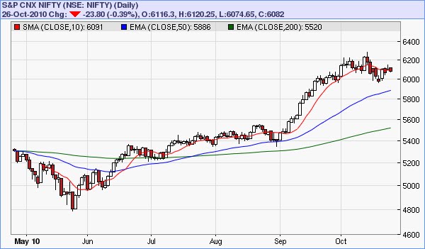
The longer the moving average, the more the lag. A 10-day moving average will hug prices quite closely and turn shortly after prices turn. Short moving averages are like speed boats - nimble and quick to change. In contrast, a 200-day moving average contains lots of past data that slows it down. Longer moving averages are like ocean tankers - lethargic and slow to change. It takes a larger and longer price movement for a 200-day moving average to change course. Below chart shows the S&P CNX Nifty with a 10-day SMA closely following prices and a 200-day EMA grinding higher. The 50-day EMA fits somewhere between the 10 and 200 day moving averages when it comes to the lag factor.

Lengths and Timeframes

The length of the moving average depends on the analytical objectives. Short moving averages (5-20 periods) are best suited for short-term trends and trading. Chartists interested in medium-term trends would opt for longer moving averages that might extend 20-60 periods. Long-term investors will prefer moving averages with 100 or more periods.

Some moving average lengths are more popular than others. The 200-day moving average is perhaps the most popular. Because of its length, this is clearly a long-term moving average. Next, the 50-day moving average is quite popular for the medium-term trend. Many chartists use the 50-day and 200-day moving averages together. Short-term, a 10-day moving average was quite popular in the past because it was easy to calculate. One simply added the numbers and moved the decimal point.

BEARISH CONTINUATION CANDLESTICK PATTERNS

BEARISH CONTINUATION PATTERNS

BEARISH REVERSAL CANDLESTICK PATTERNS



BEARISH REVERSAL PATTERNS



BULLISH CONTINUATION CANDLESTICK PATTERNS

BULLISH CONTINUATION PATTERNS

CANDLESTICKS PATTERN - BULLISH DRAGONFLY DOJI

BULLISH DRAGONFLY DOJI

Type:	Reversal
Relevance:	Bullish
Prior Trend:	Bearish
Reliability:	Medium
Confirmation:	Suggested
No. of Sticks:	1

The Bullish Dragonfly Doji Pattern is a single candlestick pattern that occurs at the bottom of a trend or during a downtrend. The Bullish Dragonfly Doji Pattern is very similar to the Bullish Hammer Pattern mentioned above. The distinction between the two is if there is a body or not. In case of Bullish Dragonfly Doji Pattern, the opening and closing prices are identical and there is no body. On the other hand the Bullish Hammer Pattern has a small real body at the upper end of the trading range.

Recognition Criteria:

1. There is an overall downtrend in the market.
2. Then we see a Doji at the upper end of the trading range.
3. The doji has an extremely long lower shadow.
4. However the doji does not have any upper shadow.

Explanation:

The market is in an overall bearish mood characterized by a downtrend. Then market opens and sells off sharply. However, the sell-off is suddenly abated and the prices reverse direction and start going up for the rest of the day closing at or near the day’s high thus leading to the long lower shadow. The failure of the market to continue in the selling side reduces the bearish sentiment. Now the shorts are increasingly uneasy with their bearish positions. If the market opens higher next day, many shorts will have a strong incentive to cover their short positions.

Important Factors:

The Bullish Dragonfly Doji Pattern is a more bullish signal than a Bullish Hammer Pattern. Its reliability is also higher than the Bullish Hammer Pattern. 

However, a confirmation of the trend reversal implied by this pattern by either a white candlestick, a large gap up or a higher close on the next trading day is still suggested, to be on the safe side.